【OpenCV3】直方图、频域

本文图像素材：

lena

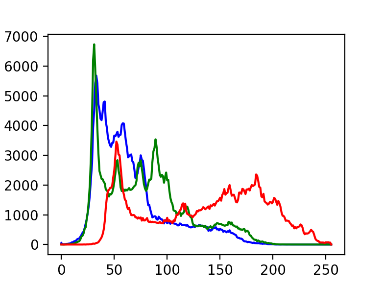
直方图

画出直方图

img = cv2.imread("a2.jpeg")
plt.hist(img.ravel(), 256)
plt.show()

或者用cv2自带的工具画图

histb = cv2.calcHist(imges=[img], channels=[0], mask=None, histSize=[256], ranges=[0, 255])
histg = cv2.calcHist([img], [1], None, [256], [0, 255])
histr = cv2.calcHist([img], [2], None, [256], [0, 255])
plt.plot(histb, color='b')
plt.plot(histg, color='g')
plt.plot(histr, color='r')
plt.show()

hist

参数

images: 图像，格式为 uint8 或 ﬂoat32。
channels: 如果入图像是灰度图它的值就是 [0]；如果是彩色图像的传入的参数可以是 [0][1][2] 它们分别对应着 BGR。
mask: 掩模图像。统整幅图像的直方图就把它为 None。但是如果你想统图像某一分的直方图的你就制作一个掩模图像并使用它。
histSize:BIN 的数目。也应用中括号括来。
ranges: 像素值范围常为 [0 256]

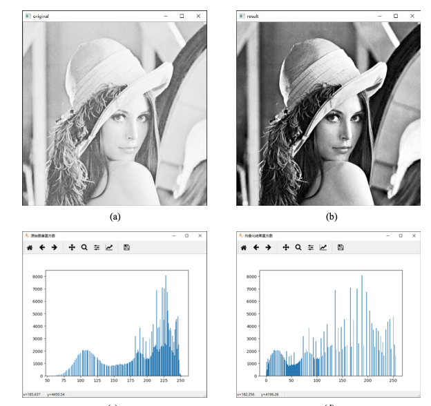
直方图均衡化

import cv2
import matplotlib.pyplot as plt

# -----------读取原始图像---------------
img = cv2.imread('a2.jpeg', cv2.IMREAD_GRAYSCALE)
# -----------直方图均衡化处理---------------
equ = cv2.equalizeHist(img)
# -----------显示均衡化前后的图像---------------
cv2.imshow("original", img)
cv2.imshow("result", equ)
# -----------显示均衡化前后的直方图---------------
plt.figure("原始图像直方图")  # 构建窗口
plt.hist(img.ravel(), 256)
plt.figure("均衡化结果直方图")
# 构建新窗口
plt.hist(equ.ravel(), 256)
# ----------等待释放窗口---------------------
cv2.waitKey()
cv2.destroyAllWindows()

equalize_hist

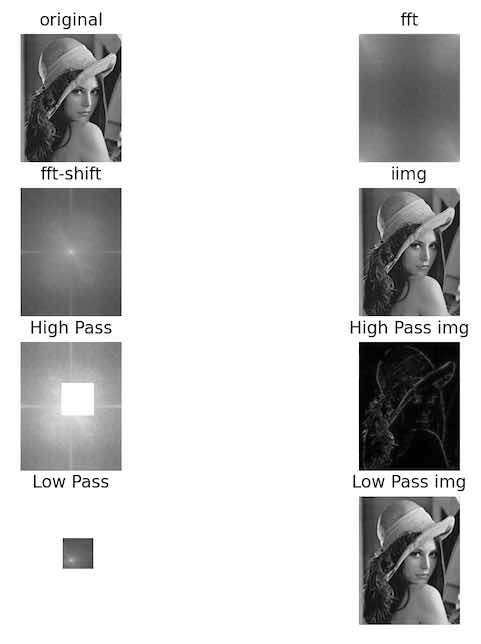
傅立叶变换

numpy 实现

返回值 = np.fft.fft2(原始图像)

# 零频率分量位于频域图像的左上角

# 为了便于观察，通常会使用numpy.fft.fftshift()函数将零频率成分 移动到频域图像的中心位置

# 对图像进行傅里叶变换后，得到的是一个复数数组。为了显示为图像，需要将它们的值调 整到[0, 255]的灰度空间内，使用的公式为:
# 像素新值=20*np.log(np.abs(频谱值))

高通滤波器和低通滤波器

允许低频信号通过的滤波器称为低通滤波器。低通滤波器使高频信号衰减而对低频信号放行，会使图像变模糊。
允许高频信号通过的滤波器称为高通滤波器。高通滤波器使低频信号衰减而让高频信号通过，将增强图像中尖锐的细节，但是会导致图像的对比度降低。

例子：傅立叶变换+逆变换的可视化

import cv2
import numpy as np
import matplotlib.pyplot as plt

img = cv2.imread('lena.jpeg', cv2.IMREAD_GRAYSCALE)
f = np.fft.fft2(img)
fshift = np.fft.fftshift(f)
magnitude_spectrum = 20 * np.log(np.abs(fshift))

fig, ax = plt.subplots(4, 2)

# %%傅立叶变换
# 原图
ax[0, 0].imshow(img, cmap='gray')
ax[0, 0].set_title('original', loc='center')
ax[0, 0].axis('off')

# fft
ax[0, 1].imshow(20 * np.log(np.abs(f)), cmap='gray')
ax[0, 1].set_title('fft', loc='center')
ax[0, 1].axis('off')

# fft-shift
ax[1, 0].imshow(magnitude_spectrum, cmap='gray')
ax[1, 0].set_title('fft-shift', loc='center')
ax[1, 0].axis('off')

# 逆变换回去
ishift = np.fft.ifftshift(fshift)
iimg = np.fft.ifft2(ishift)
iimg = np.abs(iimg)
ax[1, 1].imshow(iimg, cmap='gray')
ax[1, 1].set_title('iimg', loc='center')
ax[1, 1].axis('off')

# %% 高通滤波：把低频部分（100长度）归零
rows, cols = img.shape
center_row, center_col = int(rows / 2), int(cols / 2)
fshift_high = fshift.copy()
fshift_high[center_row - 100:center_col + 100, center_row - 100:center_col + 100] = 0
ax[2, 0].imshow(20 * np.log(np.abs(fshift_high)), cmap='gray')
ax[2, 0].set_title('High Pass', loc='center')
ax[2, 0].axis('off')

ishift_high = np.fft.ifftshift(fshift_high)
iimg_high = np.fft.ifft2(ishift_high)
iimg_high = np.abs(iimg_high)
ax[2, 1].imshow(iimg_high, cmap='gray')
ax[2, 1].set_title('High Pass img', loc='center')
ax[2, 1].axis('off')

# %% 低通滤波：把低频部分（100长度）归零
rows, cols = img.shape
center_row, center_col = int(rows / 2), int(cols / 2)
fshift_low = np.zeros_like(fshift)

fshift_low[center_row - 100:center_col + 100, center_row - 100:center_col + 100] \
    = fshift[center_row - 100:center_col + 100, center_row - 100:center_col + 100]
ax[3, 0].imshow(20 * np.log(np.abs(fshift_low)), cmap='gray')
ax[3, 0].set_title('Low Pass', loc='center')
ax[3, 0].axis('off')

ishift_low = np.fft.ifftshift(fshift_low)
iimg_low = np.fft.ifft2(ishift_low)
iimg_low = np.abs(iimg_low)
ax[3, 1].imshow(iimg_low, cmap='gray')
ax[3, 1].set_title('Low Pass img', loc='center')
ax[3, 1].axis('off')

plt.show()

fft

cv2实现傅立叶变换

cv2.dft
cv2.idft

霍夫变换

功能：基于 二值化图 中，寻找简单的图形（例如直线、圆）

接受二值化图

原理：

可以建立一个从原图（笛卡尔空间）向霍夫空间的映射。例如，
- 把原图的一条直线 $y=kx+b$ 映射为霍夫空间的一个点 $(k, b)$
- 把原图中的一个点 (x_0, y_0) 映射为霍夫空间的一个直线 $(k, b):y_0=kx_0+b$
所以，如果原图某条直线经过了n个点，那么在霍夫空间中对应的点上有n个直线。
寻找霍夫空间中多条线汇成的点，即可得到原图中的文件
改进：笛卡尔坐标系无法处理垂直线，于是使用极坐标 $r=x\cos\theta+y\sin\theta$

lines=cv2.HoughLines(image, rho, theta, threshold)
# tho： r的像素精度，一般为0
# theta： 角度的精度
# threshold 阈值，值越少，得到的直线越多
# lines：多对浮点数，即 (r,theta)

改进，可以有以下参数：

直线的最小长度。如果直线很短，即使直线上有很多像素点，也不当做直线
允许最大像素间距。如果像素点之间的距离很远，也不当做直线。

lines =cv2.HoughLinesP(image, rho, theta, threshold, minLineLength,
maxLineGap)
# tho： r的像素精度，一般为0
# theta： 角度的精度
# threshold 阈值，值越少，得到的直线越多
# minLineLength：直线的最小长度，默认0
# maxLineGap：最小间隔，默认0
# lines：多对浮点数，即 (r,theta)

霍夫变换提取直线

输入素材：

houghlines

import cv2
import numpy as np
import matplotlib.pyplot as plt

img = cv2.imread('houghlines2.jpg', -1)
gray = cv2.cvtColor(img, cv2.COLOR_BGR2GRAY)
edges = cv2.Canny(gray, 50, 150, apertureSize=3)
orgb = cv2.cvtColor(img, cv2.COLOR_BGR2RGB)
oShow = orgb.copy()
lines = cv2.HoughLinesP(edges, 1, np.pi / 180, 1, minLineLength=100, maxLineGap=10)
for line in lines:
    x1, y1, x2, y2 = line[0]
    cv2.line(orgb, (x1, y1), (x2, y2), (255, 0, 0), 5)
plt.subplot(121)
plt.imshow(oShow)
plt.axis('off')
plt.subplot(122)
plt.imshow(orgb)
plt.axis('off')

houghlines_res

霍夫变换提取圆

hough_circle

import cv2
import numpy as np
import matplotlib.pyplot as plt

# hough_circle
img = cv2.imread('hough_circle.jpeg', 0)
imgo = cv2.imread('hough_circle.jpeg', -1)
o = cv2.cvtColor(imgo, cv2.COLOR_BGR2RGB)
oshow = o.copy()
img = cv2.medianBlur(img, 5)
circles = cv2.HoughCircles(img, cv2.HOUGH_GRADIENT, dp=1, minDist=300,
                           param1=50, param2=47,
                           minRadius=100, maxRadius=200)

# minDist:圆心间的最小间距。该值被作为阈值使用，如果存在圆心间距离小于该值的 多个圆，则仅有一个会被检测出来。
# param1:该参数是缺省的，在缺省时默认值为 100。它对应的是 Canny 边缘检测器的高阈值
# param2:圆心位置必须收到的投票数
# minRadius:圆半径的最小值
# maxRadius:圆半径的最大值
# circles:圆心坐标和半径

circles = np.uint16(np.around(circles))
for i in circles[0, :]:
    cv2.circle(o, (i[0], i[1]), i[2], (255, 0, 0), 12)
    cv2.circle(o, (i[0], i[1]), 2, (255, 0, 0), 12)
plt.subplot(121)
plt.imshow(oshow)
plt.axis('off')
plt.subplot(122)
plt.imshow(o)
plt.axis('off')

hough_circle

分水岭算法

略

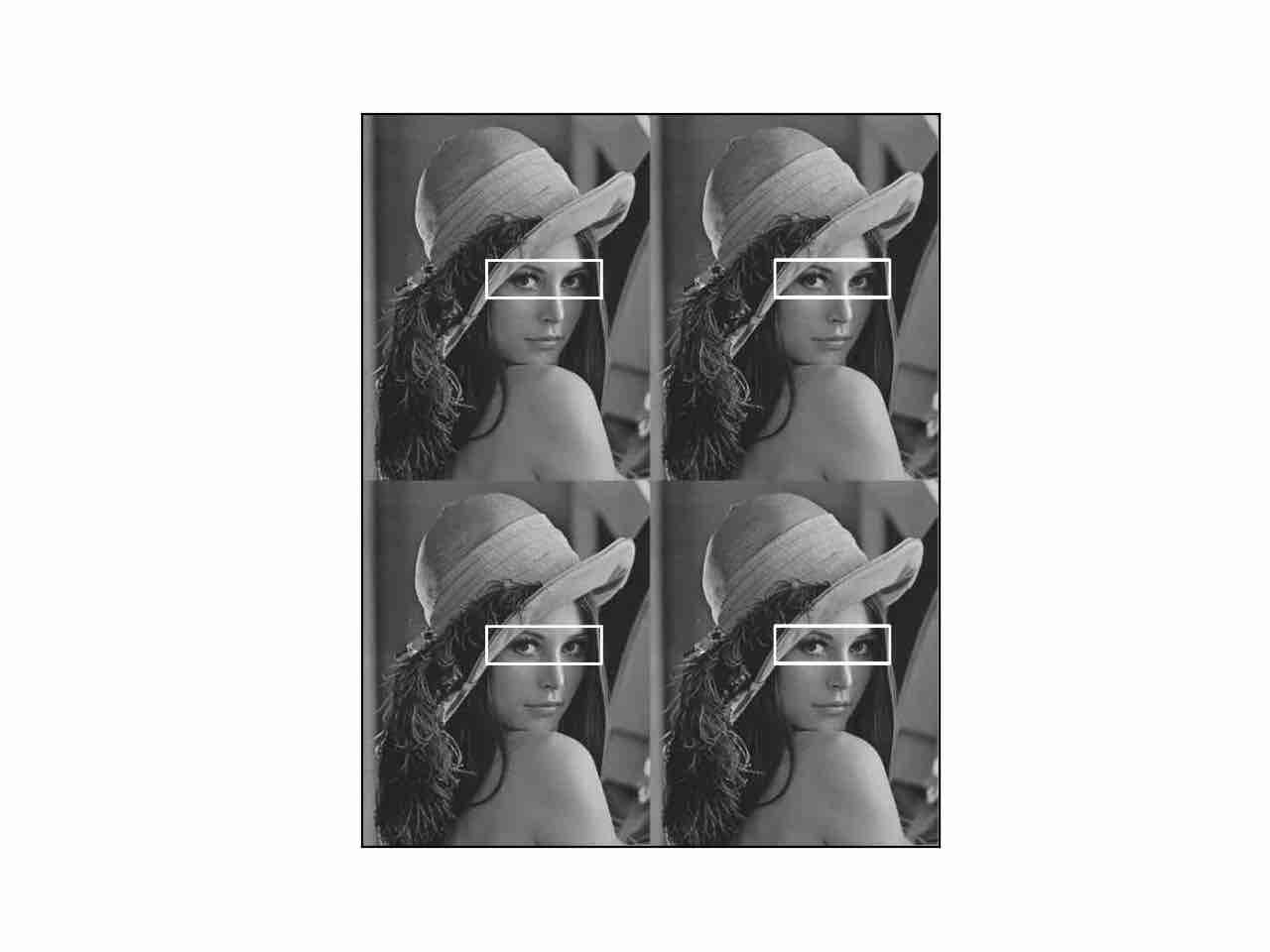
模版匹配

就是在一个图中，找另一个图.

原理：暴力遍历，每次遍历计算像素值差的方差（或平均方差、标准化方差等等，都差不多）
场景：两张图像素值点能对的上。（也就是说，不能经过放大和缩小，否则都会无法提取）

素材：

lena2

lena2_eye

代码：（展示多匹配）

import cv2
import numpy as np
from matplotlib import pyplot as plt

img = cv2.imread('lena2.png', cv2.IMREAD_GRAYSCALE)
template = cv2.imread('lena2Temp.png', cv2.IMREAD_GRAYSCALE)
w, h = template.shape[::-1]
res = cv2.matchTemplate(img, template, cv2.TM_CCOEFF_NORMED)
threshold = 0.9
loc = np.where(res >= threshold)
for pt in zip(*loc[::-1]):
    cv2.rectangle(img, pt, (pt[0] + w, pt[1] + h), 255, 1)
plt.imshow(img, cmap='gray')
plt.xticks([]), plt.yticks([])

结果：

lena2_res

应用：模版被缩放过

import numpy as np
import cv2

template = cv2.imread('template.jpg') # template image
image_o = cv2.imread('image.jpg') # image

template = cv2.cvtColor(template, cv2.COLOR_BGR2GRAY)
image = cv2.cvtColor(image_o, cv2.COLOR_BGR2GRAY)

loc = False
threshold = 0.9
w, h = template.shape[::-1]
for scale in np.linspace(0.2, 1.0, 20)[::-1]:

    resized = cv2.resize(template, dsize=(w, h))
    w, h = resized.shape[::-1]
    res = cv2.matchTemplate(image, resized, cv2.TM_CCOEFF_NORMED)

    loc = np.where(res >= threshold)
    if len(list(zip(*loc[::-1]))) > 0:
        break

if loc and len(list(zip(*loc[::-1]))) > 0:
    for pt in zip(*loc[::-1]):
        cv2.rectangle(image_o, pt, (pt[0] + w, pt[1] + h), (0, 0, 255), 2)

cv2.imshow('Matched Template', image_o)
cv2.waitKey(0)
cv2.destroyAllWindows()

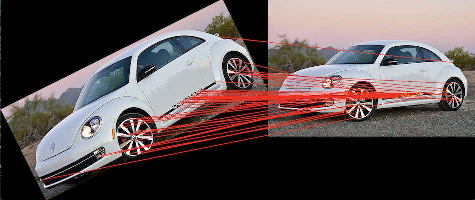
寻找映射关系

demo:映射关系可视化

import numpy as np
import cv2

img1 = cv2.imread('small.png', cv2.IMREAD_COLOR)  # queryImage
img2 = cv2.imread('big.jpeg', cv2.IMREAD_COLOR)  # trainImage


def drawMatches(img1, kp1, img2, kp2, matches):
    rows1 = img1.shape[0]
    cols1 = img1.shape[1]
    rows2 = img2.shape[0]
    cols2 = img2.shape[1]

    out = np.zeros((max([rows1, rows2]), cols1 + cols2, 3), dtype='uint8')

    # 拼接图像
    out[:rows1, :cols1] = img1
    out[:rows2, cols1:] = img2

    for match in matches:
        (x1, y1) = kp1[match.queryIdx].pt
        (x2, y2) = kp2[match.trainIdx].pt
        # 绘制匹配点
        cv2.circle(out, (int(x1), int(y1)), 4, (255, 255, 0), 1)
        cv2.circle(out, (int(x2) + cols1, int(y2)), 4, (0, 255, 255), 1)

        cv2.line(out, (int(x1), int(y1)), (int(x2) + cols1, int(y2)), (0, 0, 255), 2)

    return out


detector = cv2.ORB_create()

kp1 = detector.detect(img1, None)
kp2 = detector.detect(img2, None)
kp1, des1 = detector.compute(img1, kp1)
kp2, des2 = detector.compute(img2, kp2)

bf = cv2.BFMatcher(cv2.NORM_HAMMING, crossCheck=True)
matches = bf.match(des1, des2)
img3 = drawMatches(img1, kp1, img2, kp2, matches[:50])

cv2.imshow('orbTest', img3)
cv2.waitKey(0)

orb

关于 matches

matches 是一个列表，m = matches[0] 是一个 <DMatch> 对象
m.queryIdx 和 m.trainIdx 是一对整数，代表两个点的标号
m.distance 是两个点之间的距离（不相似度）
m.imgIdx ???暂不知道啥意思，全是0

关于 kp1[i]

是一个关键点的列表。kp = kp[0] 是一个 <KeyPoint> 对象
kp1[m.queryIdx].pt, kp2[m.trainIdx].pt 表示点的坐标
kp.pt 坐标值
kp.size 临域直径
kp.angle 方向角度，负值表示不使用
kp.octave 所在图像金字塔的组
kp.class_id 用于聚类的id
kp.response 不知道

不同的关键点匹配算法

cv2.FlannBasedMatcher 使用快速最近邻搜索算法（FLANN）来加速特征匹配。它可以处理大型特征集

cv2.BFMatcher 使用暴力匹配算法。它在小数据集上效果很好，但是在大型数据集上速度相对较慢。

FLANN_INDEX_KDTREE = 0
index_params = dict(algorithm=FLANN_INDEX_KDTREE, trees=5)
search_params = dict(checks=50)
flann = cv2.FlannBasedMatcher(index_params, search_params)
matches = flann.knnMatch(des1, des2, k=2)

# create BFmatcher object. Brute-Force，暴力match。
# BFMatcher有两个params
# 第一个是normType，是各点之间的距离。
# 第二个是crossCheck，是布尔逻辑值。True的时候，会两张图的点A→B和B→A各算一次。
bf = cv2.BFMatcher(cv2.NORM_HAMMING, crossCheck=True)
# bf = cv2.BFMatcher(cv2.NORM_L1, crossCheck=False)

matches = bf.match(des1, des2)
# knnmatch是只保留前若干个最佳的k个点
# 是knnMatch(des1,des2,k=2)

demo:还原

def recovery(ori_img, attacked_img, outfile_name='./recoveried.png', rate=0.7):
    img = cv2.imread(ori_img)
    img2 = cv2.imread(attacked_img)

    height = img.shape[0]
    width = img.shape[1]
    # Initiate SIFT detector
    orb = cv2.ORB_create(300)
    MIN_MATCH_COUNT = 10
    # find the keypoints and descriptors with SIFT
    kp1, des1 = orb.detectAndCompute(img, None)
    kp2, des2 = orb.detectAndCompute(img2, None)

    des1 = np.float32(des1)
    des2 = np.float32(des2)

    FLANN_INDEX_KDTREE = 0
    index_params = dict(algorithm=FLANN_INDEX_KDTREE, trees=5)
    search_params = dict(checks=50)
    flann = cv2.FlannBasedMatcher(index_params, search_params)
    matches = flann.knnMatch(des1, des2, k=2)

    # store all the good matches as per Lowe's ratio test.
    good = []
    for m, n in matches:
        if m.distance < rate * n.distance:
            good.append(m)

    if len(good) > MIN_MATCH_COUNT:
        src_pts = np.float32([kp1[m.queryIdx].pt for m in good]).reshape(-1, 1, 2)
        dst_pts = np.float32([kp2[m.trainIdx].pt for m in good]).reshape(-1, 1, 2)
        M, mask = cv2.findHomography(dst_pts, src_pts, cv2.RANSAC, 5.0)
        out = cv2.warpPerspective(img2, M, (width, height))
        cv2.imwrite(outfile_name, out)
    else:
        print("无法还原")

不同的特征提取器

cv2.ORB_create. 基于 ORB（Oriented FAST and Rotated BRIEF），它是一个基于FAST特征检测器和BRIEF描述符的改进算法，它能够在图像中检测出关键点，并提取出该点的局部特征描述子，适用于目标跟踪、图像拼接等应用领域。
cv2.SIFT_create. 基于 SIFT（Scale-Invariant Feature Transform），是一种用于在图像中检测和描述局部特征的算法。它具有尺度不变性和旋转不变性，能够检测出物体的关键点，并提取出该点的局部特征描述子，适用于目标识别、场景重建、图像匹配等应用领域。

sift = cv2.xfeatures2d.SIFT_create()

kp1, des1 = sift.detectAndCompute(img1, None)
kp2, des2 = sift.detectAndCompute(img2, None)

bf = cv2.BFMatcher()
matches = bf.knnMatch(des1, des2, k=2)

end

0x00_读论文 8

0x11_算法平台 15

0x12_Pandas与numpy 12

0x13_特征工程 4

0x21_有监督学习 21

0x22_上世纪神经网络 10

0x23_深度学习 7

0x24_NLP 13

0x25_CV 11

0x26_torch 11

0x31_降维 10

0x32_聚类 5

0x33_图模型 9

0x41_统计模型 9

0x42_概率论 7

0x43_时间序列 10

0x44_随机过程 2

0x51_代数与分析 14

0x52_方程 2

0x53_复分析与积分变换 8

0x55_数值计算 7

0x56_最优化 11

0x58_密码学 13

0x59_应用数学 9

0x60_启发式算法 8

0x70_可视化 13

0x80_数据结构与算法 17

0xa0_蒙特卡洛方法 6

0xb0_Python语法 18

0xd0_设计模式 6