【logistics】理论与实现
🗓 2017年05月07日 📁 文章归类: 0x21_有监督学习
版权声明:本文作者是郭飞。转载随意,标明原文链接即可。
原文链接:https://www.guofei.site/2017/05/07/LogisticRegression.html
logistics regression是一种典型的分类模型
logistic regression, logit regression, logit model这三个模型本质和用法非常相似,因此这里不加区分
logistic distribution
定义
CDF满足这个的随机变量叫做logistic distribution
$F(x; \mu, s) = \dfrac{1}{1+e^{-(x-\mu)/s}}$
性质
不难推导出PDF:
$f(x; \mu,s) = \dfrac {e^{-(x-\mu)/s}} {s (1+e^{-(x-\mu)/s})^2}$
logistic regression
模型
$P(Y=1 \mid x)=\dfrac{\exp(wx)}{1+\exp(wx)}$
$P(Y=0 \mid x)=\dfrac{1}{1+\exp(wx)}$
算法
求参数的方法,就是经典的 MLE (极大似然估计)方法。
先求似然函数,
$l(w;x)=\prod \limits_{i=1}^N [P(Y=1|x)]^{y_i} [P(Y=0|x)]^{1-y_i}$
取对数后求$argmax \ln l(w)$
这是一个 凸函数 ,(凸函数的知识参见我的另一篇博文最优化方法理论篇)
由于是一个凸函数,可以用导数值为0确定最大值点,还可以用梯度下降法迭代求解最大值点。
推导似然函数:
令$L(w;x)=\ln l(w;x)$
$L(w;x)=\sum \limits_{i=1}^N (y_i w x_i - \ln (1+e^{wx_i}))$
w和x都是向量。下面研究向量的第j个分量
偏导数为:
$\dfrac{\partial L(w;x)}{\partial w_j} = \sum \limits_{i=1}^N (y_i x_{ij} - \dfrac{e^{wx_i}x_{ij}}{1+e^{wx_i}}) = \sum \limits_{i=1}^N (y_i - \dfrac{e^{w x_i}}{1+e^{wx_i}})x_{ij}$
- 令导数为0,遗憾的是无法求出解析解。
- 因此用梯度法可以求解
Python实现(自己编程)
梯度法
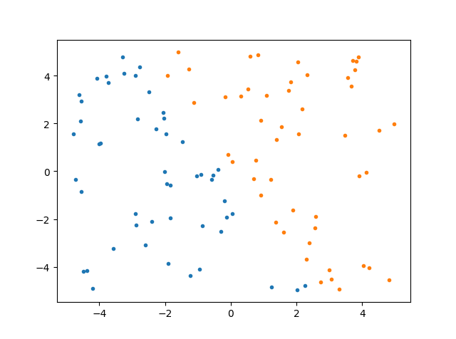
首先生成模拟数据
import numpy as np
import pandas as pd
import matplotlib.pyplot as plt
data = np.random.uniform(low=-5, high=5, size=(100, 2))
data=pd.DataFrame(data)
mask = (data.iloc[:, 0] + 0.5* data.iloc[:, 1])<0
data['y']=mask*1

data1 = data[data.iloc[:, 2] == 1] #为了画图,两类不同颜色
data2 = data[data.iloc[:, 2] == 0]
plt.plot(data1.iloc[:, 0], data1.iloc[:, 1], '.')
plt.plot(data2.iloc[:, 0], data2.iloc[:, 1], '.')
plt.show()
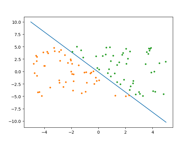
迭代求解:
alpha = 0.001 # 步长
step = 500   # 总共的迭代次数
m, n = data.shape
weights = np.ones((n, 1))

data_x = np.concatenate((np.ones((m, 1)), np.array(data.iloc[:, :2])), axis=1)  # 去掉y列,并添加全1的第一列
target = np.array(data.iloc[:, 2])
target.shape = -1, 1


def logistic(wTx):
    return 1 / (1 + np.exp(-wTx))


for i in range(step):
    wTx = np.dot(data_x, weights)
    output = logistic(wTx)
    errors = target - output
    weights = weights + alpha * np.dot(data_x.T, errors)

X = np.linspace(-5, 5, 100)
Y = -(weights[0] + X * weights[1]) / weights[2]


plt.plot(X, Y)
plt.plot(data1.iloc[:, 0], data1.iloc[:, 1], '.')
plt.plot(data2.iloc[:, 0], data2.iloc[:, 1], '.')
plt.show()
随机梯度下降法
随机梯度下降法并没有引入新理论,解决的主要问题是步长alpha的问题。
alpha太大,容易越过极值点,导致震荡不收敛。
alpha太小,收敛速度会降低。
算法的伪代码是这样的:
for 第i次迭代
    for 第j次收取
        alpha=2/(1+i+j)+0.001
        从全部样本中随机抽取样本,梯度下降,步长为alpha
Python实现(sklearn)
step1:建立模型
from sklearn.datasets import load_iris
dataset=load_iris()

from sklearn import linear_model
clf=linear_model.LogisticRegression()
clf.fit(dataset.data,dataset.target)
关于参数的选择,一定要看sklearn官网1
step2:模型使用
clf.predict(dataset.data)#判断数据属于哪个类别
clf.predict_proba(dataset.data)#判断属于各个类别的概率
clf.score(dataset.data,dataset.target)#准确率


clf.coef_ #系数
clf.intercept_ #截距
clf.n_iter_ #迭代次数
备注
筛选+回归
用到sklearn中的两个模型
RandomizedLogisticRegression用来筛选变量
LogisticRegression用来做逻辑回归
step1:用RandomizedLogisticRegression筛选有效变量
from sklearn.linear_model import LogisticRegression as LR
from sklearn.linear_model import RandomizedLogisticRegression as RLR
rlr = RLR() #建立随机逻辑回归模型,用于筛选变量
rlr.fit(x, y) #训练模型
rlr.get_support() #获取特征筛选结果,是一个boll类型的array
rlr.scores_#各个特征的分数,是1darray
print('通过随机逻辑回归模型筛选特征结束。')
print('有效特征为:%s' % ','.join(x.columns[rlr.get_support()]))
step2:用LogisticRegression做逻辑回归
x_new = x[x.columns[rlr.get_support()]] #筛选好特征
lr = LR() #建立逻辑回归模型
lr.fit(x_new, y) #用筛选后的特征数据来训练模型
print('逻辑回归模型训练结束。')
print('模型的平均正确率为:%s' % lr.score(x_new, y)) #给出模型的平均正确率,本例为81.4%
参考文献
您的支持将鼓励我继续创作!