【最优化】scipy.optimize.fmin
🗓 2017年06月06日 📁 文章归类: 0x56_最优化
版权声明:本文作者是郭飞。转载随意,标明原文链接即可。
原文链接:https://www.guofei.site/2017/06/06/scipyfmin.html
fmin
这部分代码借鉴了《Python科学计算》,进行了改动
import scipy.optimize as opt
import numpy as np

points = []


def obj_func(p):
    x, y = p
    z = (1 - x) ** 2 + 100 * (y - x ** 2) ** 2  # 这里可以加一项,用来做带约束
    points.append((x, y, z))
    return z


# 雅克比矩阵,也就是偏导数矩阵,有些优化方法用得到,有些用不到
def fprime(p):
    x, y = p
    dx = -2 + 2 * x - 400 * x * (y - x ** 2)
    dy = 200 * y - 200 * x ** 2
    return np.array([dx, dy])


init_point = np.array([-2, -2])

# 这两种优化方法没用到偏导
result = opt.fmin(func=obj_func, x0=init_point)  # downhill simplex algorithm
# result = opt.fmin_powell(func=obj_func, x0=init_point)  # modified Powell's method

# 用到偏导的(都不是必须传入偏导):
# result = opt.fmin_cg(f=obj_func, x0=init_point, fprime=fprime)  # nonlinear conjugate gradient algorithm
# result = opt.fmin_bfgs(f=obj_func, x0=init_point, fprime=fprime)  # BFGS algorithm
# result = opt.fmin_tnc(func=obj_func, x0=init_point, fprime=fprime)
# truncated Newton algorithm,可以传入 bounds=(min, max) 来做有约束优化
# result = opt.fmin_l_bfgs_b(func=obj_func, x0=init_point, fprime=fprime)
# L-BFGS-B algorithm,可以传入 bounds=(min, max) 来做有约束优化

# 其它
# result = opt.fmin_cobyla(func=obj_func, x0=init_point, cons=[])
# Constrained Optimization BY Linear Approximation (COBYLA) method
'''
    cons : sequence
        Constraint functions; must all be ``>=0`` (a single function
        if only 1 constraint). Each function takes the parameters `x`
        as its first argument, and it can return either a single number or
        an array or list of numbers.
'''

print(result)


# 绘图
import pylab as pl

p = np.array(points)
xmin, xmax = np.min(p[:, 0]) - 1, np.max(p[:, 0]) + 1
ymin, ymax = np.min(p[:, 1]), np.max(p[:, 1]) + 1
Y, X = np.ogrid[ymin:ymax:500j, xmin:xmax:500j]
Z = np.log10(obj_func((X, Y)))
zmin, zmax = np.min(Z), np.max(Z)

pl.imshow(Z, extent=(xmin, xmax, ymin, ymax), origin="bottom", aspect="auto")
pl.plot(p[:, 0], p[:, 1])
pl.scatter(p[:, 0], p[:, 1], c=range(len(p)))
pl.xlim(xmin, xmax)
pl.ylim(ymin, ymax)
pl.show()
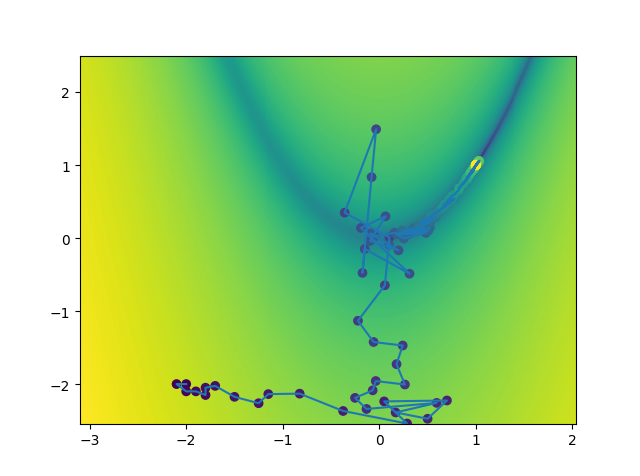
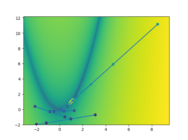
下面这2个优化方法的展示:
fmin:
fmin_tnc:
opt.minimize
opt.minimize 这个函数将众多优化算法打包到一起
opt.minimize(fun, x0, args=(), method=None, jac=None, hess=None, hessp=None, bounds=None, constraints=(), tol=None, callback=None, options=None)
'''
minimize f(x) subject to

g_i(x) >= 0,  i = 1,...,m
h_j(x)  = 0,  j = 1,...,p


fun : callable
  The objective function to be minimized. Must be in the form
  ``f(x, *args)``. The optimizing argument, ``x``, is a 1-D array
  of points, and ``args`` is a tuple of any additional fixed parameters
  needed to completely specify the function.

x0 : ndarray
  Initial guess. ``len(x0)`` is the dimensionality of the minimization
  problem.

method : str or callable, optional
  Type of solver. 内容比较多,在下面一个章节详解

  If not given, chosen to be one of ``BFGS``, ``L-BFGS-B``, ``SLSQP``,
  depending if the problem has constraints or bounds.

jac : bool or callable, optional
  Jacobian (gradient) of objective function. Only for CG, BFGS,
  Newton-CG, L-BFGS-B, TNC, SLSQP, dogleg, trust-ncg, trust-krylov,
  trust-region-exact.
  If `jac` is a Boolean and is True, `fun` is assumed to return the
  gradient along with the objective function. If False, the
  gradient will be estimated numerically.
  `jac` can also be a callable returning the gradient of the
  objective. In this case, it must accept the same arguments as `fun`.

hess, hessp : callable, optional
  Hessian (matrix of second-order derivatives) of objective function or
  Hessian of objective function times an arbitrary vector p.  Only for
  Newton-CG, dogleg, trust-ncg, trust-krylov, trust-region-exact.
  Only one of `hessp` or `hess` needs to be given.  If `hess` is
  provided, then `hessp` will be ignored.  If neither `hess` nor
  `hessp` is provided, then the Hessian product will be approximated
  using finite differences on `jac`. `hessp` must compute the Hessian
  times an arbitrary vector.

bounds : sequence, optional
Bounds for variables (only for L-BFGS-B, TNC and SLSQP).
  ``(min, max)`` pairs for each element in ``x``, defining
  the bounds on that parameter. Use None for one of ``min`` or
  ``max`` when there is no bound in that direction.
  constraints : dict or sequence of dict, optional
  Constraints definition (only for COBYLA and SLSQP).
  Each constraint is defined in a dictionary with fields:

      type : str
          Constraint type: 'eq' for equality, 'ineq' for inequality.
      fun : callable
          The function defining the constraint.
      jac : callable, optional
          The Jacobian of `fun` (only for SLSQP).
      args : sequence, optional
          Extra arguments to be passed to the function and Jacobian.

  Equality constraint means that the constraint function result is to
  be zero whereas inequality means that it is to be non-negative.
  Note that COBYLA only supports inequality constraints.

tol : float, optional
  Tolerance for termination. For detailed control, use solver-specific
  options.
  options : dict, optional
  A dictionary of solver options. All methods accept the following
  generic options:

      maxiter : int
          Maximum number of iterations to perform.
      disp : bool
          Set to True to print convergence messages.

  For method-specific options, see :func:`show_options()`.

callback : callable, optional
  Called after each iteration, as ``callback(xk)``, where ``xk`` is the
  current parameter vector.

Returns
-------
res : OptimizeResult
The optimization result represented as a ``OptimizeResult`` object.
Important attributes are: ``x`` the solution array, ``success`` a
Boolean flag indicating if the optimizer exited successfully and
``message`` which describes the cause of the termination. See
`OptimizeResult` for a description of other attributes.
'''
Notes
This section describes the available solvers that can be selected by the ‘method’ parameter. The default method is BFGS.
1. Unconstrained minimization
Nelder-Meaduses the Simplex algorithm . This algorithm is robust in many applications. However, if numerical computation of derivative can be trusted, other algorithms using the first and/or second derivatives information might be preferred for their better performance in general.Powellis a modification of Powell’s method which is a conjugate direction method. It performs sequential one-dimensional minimizations along each vector of the directions set (direcfield inoptionsandinfo), which is updated at each iteration of the main minimization loop. The function need not be differentiable, and no derivatives are taken.CGuses a nonlinear conjugate gradient algorithm by Polak and Ribiere, a variant of the Fletcher-Reeves method. Only the first derivatives are used.BFGSuses the quasi-Newton method of Broyden, Fletcher, Goldfarb, and Shanno (BFGS). It uses the first derivatives only. BFGS has proven good performance even for non-smooth optimizations. This method also returns an approximation of the Hessian inverse, stored ashess_invin the OptimizeResult object.Newton-CGuses a Newton-CG algorithm (also known as the truncated Newton method). It uses a CG method to the compute the search direction. See also TNC method for a box-constrained minimization with a similar algorithm. Suitable for large-scale problems.dogleguses the dog-leg trust-region algorithm for unconstrained minimization. This algorithm requires the gradient and Hessian; furthermore the Hessian is required to be positive definite.trust-ncguses the Newton conjugate gradient trust-region algorithm for unconstrained minimization. This algorithm requires the gradient and either the Hessian or a function that computes the product of the Hessian with a given vector. Suitable for large-scale problems.trust-krylovuses the Newton GLTR trust-region algorithm for unconstrained minimization. This algorithm requires the gradient and either the Hessian or a function that computes the product of the Hessian with a given vector. Suitable for large-scale problems. On indefinite problems it requires usually less iterations than thetrust-ncgmethod and is recommended for medium and large-scale problems.trust-exactis a trust-region method for unconstrained minimization in which quadratic subproblems are solved almost exactly. This algorithm requires the gradient and the Hessian (which is not required to be positive definite). It is, in many situations, the Newton method to converge in fewer iteraction and the most recommended for small and medium-size problems.
2. Constrained minimization
L-BFGS-Buses the L-BFGS-B algorithm for bound constrained minimization.TNCuses a truncated Newton algorithm to minimize a function with variables subject to bounds. This algorithm uses gradient information; it is also called Newton Conjugate-Gradient. It differs from the Newton-CG method described above as it wraps a C implementation and allows each variable to be given upper and lower bounds.COBYLAuses the Constrained Optimization BY Linear Approximation (COBYLA) method. The algorithm is based on linear approximations to the objective function and each constraint. The method wraps a FORTRAN implementation of the algorithm. The constraints functions ‘fun’ may return either a single number or an array or list of numbers.SLSQPuses Sequential Least SQuares Programming to minimize a function of several variables with any combination of bounds, equality and inequality constraints. The method wraps the SLSQP Optimization subroutine originally implemented by Dieter Kraft . Note that the wrapper handles infinite values in bounds by converting them into large floating values.
3. Custom minimizers
It may be useful to pass a custom minimization method, for example when using a frontend to this method such as scipy.optimize.basinhopping or a different library. You can simply pass a callable as the method parameter.
The callable is called as method(fun, x0, args, **kwargs, **options) where kwargs corresponds to any other parameters passed to minimize (such as callback, hess, etc.), except the options dict, which has its contents also passed as method parameters pair by pair. Also, if jac has been passed as a bool type, jac and fun are mangled so that fun returns just the function values and jac is converted to a function returning the Jacobian. The method shall return an OptimizeResult object.
The provided method callable must be able to accept (and possibly ignore) arbitrary parameters; the set of parameters accepted by minimize may expand in future versions and then these parameters will be passed to the method. You can find an example in the scipy.optimize tutorial.
总结就是这样:
| 算法 | 简介 | 特点 | jac(梯度) | hess | bounds |
|---|---|---|---|---|---|
| Nelder-Mead | 单纯形法 | 稳定,如果微分可信,推荐其他算法 | 无约束 | ||
| Powell | 每次搜索一个维度 | 不必可微 | 不需要 | 不需要 | 无约束 |
| CG | 非线性共轭方向 | 需要 | 不需要 | 无约束 | |
| BFGS | quasi-Newton method of Broyden | 对于不平滑问题也表现良好 | 需要 | 不需要 | 无约束 |
| Newton-CG | 使用CG算法确定方向 | 适合large-scale problems | 需要 | 需要 | 无约束 |
| dogleg | dog-leg trust-region algorithm | 需要 | 需要 | 无约束算法 | |
| trust-ncg | ewton conjugate gradient trust-region algorithm | 适合large-scale problems | 需要 | 需要(或者Hessian的积) | 无约束算法 |
| trust-krylov | 适合large-scale problems, 比trust-ncg迭代次数少 | 需要 | 需要(或者Hessian的积) | 无约束算法 | |
| trust-exact | 需要 | 需要(但并不要求正定) | 无约束算法 | ||
| L-BFGS-B | 需要 | 不需要 | 有约束 | ||
| TNC | truncated Newton algorithm | 需要 | 不需要 | 有约束 | |
| COBYLA | Constrained Optimization BY Linear Approximation method | 不需要 | 有约束 | ||
| SLSQP | Sequential Least SQuares Programming | 需要 | 不需要 | 有约束 |
注1:(如果jac和hess不给定的话,会用数值方法估算)
注2:默认是BFGS, L-BFGS-B, SLSQP(具体哪个取决于入参)
4. 附:Jacobian 矩阵和 Hessian 矩阵
Jacobian 矩阵:
\(\dfrac{\partial (y_1,...,y_m)}{\partial(x_1,...,x_n)}=
\left[ \begin{array}{ccc}
\dfrac{\partial y_1}{\partial x_1}&...&\dfrac{\partial y_1}{\partial x_n}\\
...\\
\dfrac{\partial y_m}{\partial x_1}&...&\dfrac{\partial y_m}{\partial x_n}
\end{array}\right]\)
Hessian 矩阵:
\(G=\left[ \begin{array}{ccc}
\dfrac{\partial^2 f}{\partial x_1^2}&\dfrac{\partial^2 f}{\partial x_1x_2}&...&\dfrac{\partial f^2}{\partial x_1 \partial x_n}\\
\dfrac{\partial^2 f}{\partial x_1 x_2}&\dfrac{\partial^2 f}{\partial x_2^2}&...&\dfrac{\partial f^2}{\partial x_2 \partial x_n}\\
...\\
\dfrac{\partial^2 f}{\partial x_n x_1}&\dfrac{\partial^2 f}{\partial x_n x_2}&...&\dfrac{\partial f^2}{\partial x_n^2}
\end{array}\right]\)
多元函数的泰勒展开:
$f(X)=f(X^{(0)})+\nabla f(X^{(0)})\Delta X+0.5 \Delta X^TG(X^{(0)})\Delta X+…$
(其中,$\nabla f(x)=[\dfrac{\partial f}{\partial x_1},\dfrac{\partial f}{\partial x_2},…,\dfrac{\partial f}{\partial x_n}]$是梯度。)
opt.minimize_scalar
用于一维情况
您的支持将鼓励我继续创作!