【statsmodels】OLS最小二乘法
🗓 2019年03月03日 📁 文章归类: 0x41_统计模型
版权声明:本文作者是郭飞。转载随意,标明原文链接即可。
原文链接:https://www.guofei.site/2019/03/03/statsmodels_ols.html
几种回归模型概述
介绍一下几种与回归statistical model1有关的模型
$Y=X\beta +u$,where $u\sim N(0,\Sigma)$
- OLS : ordinary least squares for i.i.d. errors :$\Sigma=\textbf{I}$
- WLS : weighted least squares for heteroskedastic errors :$\text{diag}(\Sigma)$
- GLS : generalized least squares for arbitrary covariance :$\Sigma$
- GLSAR : feasible generalized least squares with autocorrelated AR(p) errors :$\Sigma=\Sigma\left(\rho\right)$
OLS
setp1. 载入包和数据
import numpy as np
import matplotlib.pyplot as plt
import pandas as pd
import statsmodels.formula.api as smf

df = pd.DataFrame()
df.loc[:, 'x'] = np.linspace(start=0, stop=20, num=50)
df.loc[:, 'y'] = 2 * df.x + np.random.randn(50) + 5
step2. 构建模型
lm_s = smf.ols(formula='y ~ x', data=df).fit()
step3. 预测
from statsmodels.sandbox.regression.predstd import wls_prediction_std
prstd, iv_l, iv_u = wls_prediction_std(lm_s)
#     predstd : standard error of prediction
#     interval_l, interval_u : lower und upper confidence bounds
fig, ax = plt.subplots(figsize=(8, 6))
ax.plot(df.x, df.y, 'o', label="data") # 输入样本
ax.plot(df.x, lm_s.predict(df), 'r--.', label="OLS") # 预测值
ax.plot(df.x, iv_u, 'r--') # 预测上界
ax.plot(df.x, iv_l, 'r--') # 预测下界
ax.legend(loc='best')
plt.show()
step4. 模型结果
lm_s.predict(df) # 返回预测值y,是一个array
lm_s.resid # 返回残差,是一个pd.Series
lm_s.params # 返回参数估计值,是pd.Series类型

lm_s.summary()
lm_s.rsquared #R^2
lm_s.rsquared_adj

lm_s.aic # 越低越好
lm_s.bic # 越低越好
step5. 残差分析
sm.stats.linear_rainbow(lm_s)
sm.stats.durbin_watson(lm_s.resid) #dw检验
官网上还有多种检验方法 http://www.statsmodels.org/stable/stats.html#residual-diagnostics-and-specification-tests
除此之外还有一些不常用的属性,例如自由度、似然值等等,就不摘抄了,看官网
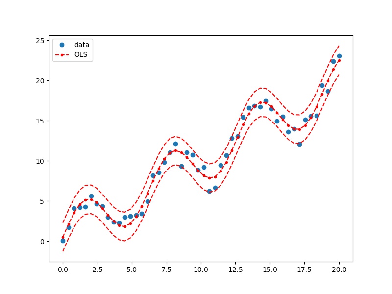
用ols做非线性回归
官网是用OLS对象做的,这里用formula重做一遍
import numpy as np
import matplotlib.pyplot as plt
import pandas as pd
import statsmodels.formula.api as smf

df = pd.DataFrame()
df.loc[:, 'x'] = np.linspace(start=0, stop=20, num=50)
df.loc[:, 'y'] = np.sin(df.x) * 3 + df.x + np.random.randn(50)

# %%
lm_s = smf.ols(formula='y ~ np.sin(x)+x', data=df).fit()

# %%

from statsmodels.sandbox.regression.predstd import wls_prediction_std

prstd, iv_l, iv_u = wls_prediction_std(lm_s)
#     predstd : standard error of prediction
#     interval_l, interval_u : lower und upper confidence bounds
fig, ax = plt.subplots(figsize=(8, 6))
ax.plot(df.x, df.y, 'o', label="data")
ax.plot(df.x, lm_s.predict(df), 'r--.', label="OLS")
ax.plot(df.x, iv_u, 'r--')
ax.plot(df.x, iv_l, 'r--')
ax.legend(loc='best')
plt.show()
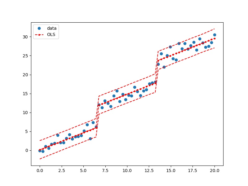
用ols做哑变量回归
import numpy as np
import matplotlib.pyplot as plt
import pandas as pd
import statsmodels.formula.api as smf

df = pd.DataFrame()
df.loc[:, 'x1'] = np.linspace(start=0, stop=20, num=60)
df.loc[:,'x2']=[0]*20+[1]*20+[2]*20
df.loc[:, 'y'] = df.x1 + 5*df.x2+np.random.randn(60)

# %%
lm_s = smf.ols(formula='y ~ np.sin(x1)+x1+x2', data=df).fit()

# %%

from statsmodels.sandbox.regression.predstd import wls_prediction_std

prstd, iv_l, iv_u = wls_prediction_std(lm_s)
#     predstd : standard error of prediction
#     interval_l, interval_u : lower und upper confidence bounds
fig, ax = plt.subplots(figsize=(8, 6))
ax.plot(df.x1, df.y, 'o', label="data")
ax.plot(df.x1, lm_s.predict(df), 'r--.', label="OLS")
ax.plot(df.x1, iv_u, 'r--')
ax.plot(df.x1, iv_l, 'r--')
ax.legend(loc='best')
plt.show()
OLS的结果检验
- F检验,用来检验方程的显著性
lm_s.f_test('x1=x2=0') - 多重共线性
lm_s.summary()
# Cond. No. 这一项太大的话,可能有多重共线性。也会在warning中列出
ridge
ols('y~x1+x2',data=df).fit_regularized(alpha=1, L1_wt=1)
TODO:LASSO, ElasticNet
R-style formulas
import statsmodels.api as sm
import statsmodels.formula.api as smf
df = sm.datasets.get_rdataset("Guerry", "HistData").data
df = df[['Lottery', 'Literacy', 'Wealth', 'Region']].dropna()
Categorical variables
res = smf.ols(formula='Lottery ~ Literacy + Wealth + Region', data=df).fit()

# C指的是Categorical variables
res = smf.ols(formula='Lottery ~ Literacy + Wealth + C(Region)', data=df).fit()
-1
# -1 指的是使 Intercept = 0
res = smf.ols(formula='Lottery ~ Literacy + Wealth + C(Region) -1 ', data=df).fit()
print(res.summary())
冒号和乘号
# “:” adds a new column to the design matrix with the product of the other two columns. “
# *” will also include the individual columns that were multiplied together:
# 所以'Lottery ~ Literacy * Wealth - 1' 相当于 'Lottery ~ Literacy + Wealth+Literacy : Wealth - 1'
res1 = smf.ols(formula='Lottery ~ Literacy : Wealth - 1', data=df).fit()
res2 = smf.ols(formula='Lottery ~ Literacy * Wealth - 1', data=df).fit()
print(res1.params)
print(res2.params)
Functions
- 直接使用numpy
res = smf.ols(formula='Lottery ~ np.log(Literacy)', data=df).fit() - 使用自定义函数
def plus_1(x):
 return x+1.0
res = smf.ols(formula='Lottery ~ plus_1(Literacy)', data=df).fit()
参考资料
您的支持将鼓励我继续创作!