描述

在随机模拟实验中，在一个给定的曲面上生成均匀随机点是一个常见的需求。
但是还没发现有太好通用的算法，这里进行一些探索。

定义

我们把问题分解成两个：

1. 在n维空间（n>=2）上的一条曲线上生成均匀随机点
2. 在n维空间（n>=3）上的一条曲面上生成均匀随机点

何为随机？

我们已经知道 同余发生器 或者 混沌迭代式 都可以生成伪随机数，这里的随机的定义保持一致。

何为均匀随机？

我们把均匀随机定义为某种度量上的随机：

• 把曲线上的均匀随机，定义为沿着曲线的长度均匀随机采样。
• 把曲面上的均匀随机，定义为沿着曲面上的面积均匀采样。

下面这个就不能定义为均匀随机采样

（不是我们要的结果）

为何不涉及其它维度？

因为都是已经解决的问题。

维度为1的曲线上的均匀分布，实际上就是一般说的均匀分布 np.random.rand() 已经有大量的讨论了。

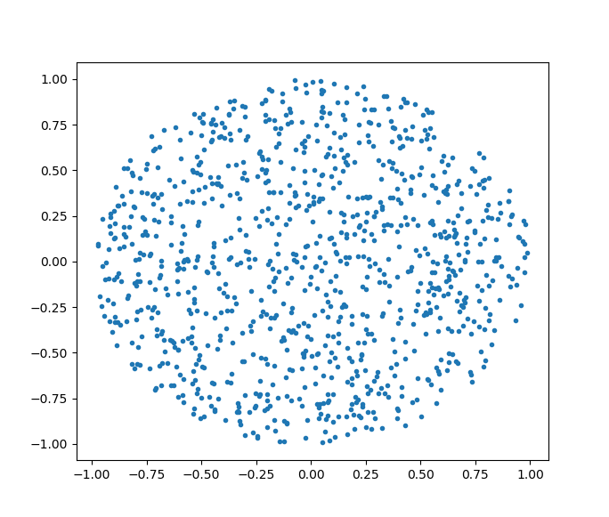
维度为2的曲面上的均匀分布，实际上就是平面上某一块区域，以二维圆面为例，算法如下：

def random_surface():
    while True:
        x, y = np.random.rand(2) * 2 - 1
        if x ** 2 + y ** 2 <= 1:
            return x, y


sample = np.array([random_surface() for i in range(1000)])
plt.plot(sample[:, 0], sample[:, 1], '.')

曲线上的均匀随机

假设曲线的表示是:
\(x=\phi(t),y=\psi(t), t\in [a,b]\)

第一类曲线积分 $\int_{a}^{b} ds$ 就是曲线的长度，
我们找到x，使得 $\dfrac{\int_{a}^{x} ds}{\int_{a}^{b} ds}=r$，其中$r\in[0,1]$
也就是$\dfrac{\int_{a}^{x} \sqrt{x’^2+y’^2} dt}{\int_{a}^{b} \sqrt{x’^2+y’^2} dt}=r, r\in[0,1]$

算法就是根据上面的方程，找到$x=f(r)$，然后生成随机的r，进而就找到x了。

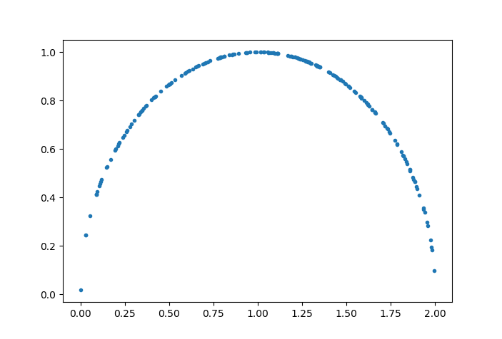
案例：圆

$x=\cos t+1,y=\sin t, t\in [0,\pi]$
$\int_0^t ds = \int_0^t \sqrt{x’^2+y’^2} dt= t$

方程是 $t/\pi =r$

代码就有了：

def random_surface():
    r = np.random.rand()
    t = r * np.pi
    x, y = np.cos(t) + 1, np.sin(t)
    return x, y


sample = np.array([random_surface() for i in range(200)])
plt.plot(sample[:, 0], sample[:, 1], '.')

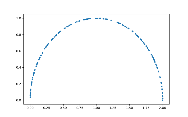
（是随机采样，所以看起来不均匀，但实际上是均匀的）

缺点与方案2

以阿基米德螺旋线$x=t\cos t, y=t\sin t$为例，
$\int_0^t ds = \int_0^t \sqrt{x’^2+y’^2} dt$
$= \int_0^t \sqrt{1+t^2}dt$
$=t/2\sqrt{1+t^2}+1/2 \ln (t+\sqrt{1+t^2})$

求积分那一步就已经有点计算量了，
解方程 $t/2\sqrt{1+t^2}+1/2 \ln (t+\sqrt{1+t^2})=r$ 更是几乎不可能。
因此必须找到一个数值方法。

import scipy.optimize as opt
import numpy as np


def func(t):
    # 被积部分
    return np.sqrt(1 + np.square(t))


from scipy import integrate

s, _ = integrate.quad(func, 0, 4 * np.pi)  # 分母

result = []
for i in range(300):
    # r = np.random.rand()
    r = i / 300
    t = opt.fsolve(lambda t: integrate.quad(func, 0, t)[0] / s - r, [0], fprime=func)
    x = t * np.cos(t)
    y = t * np.sin(t)
    result.append([x, y])

result = np.array(result)

plt.plot(result[:, 0], result[:, 1], '.')
plt.show()

• 手算出被积函数的解析形式（相对来说，不很难）
• 使用了scipy的积分算法、解方程算法（因此效率会变低）
• 为了展示是否均匀，r用均匀值，而不是随机值。在实战中改成随机值。
• fprime 是雅克比矩阵，用于解方程时，加快迭代速度，可以省略。根据Lebniz定理，雅克比矩阵正好等于被积函数。

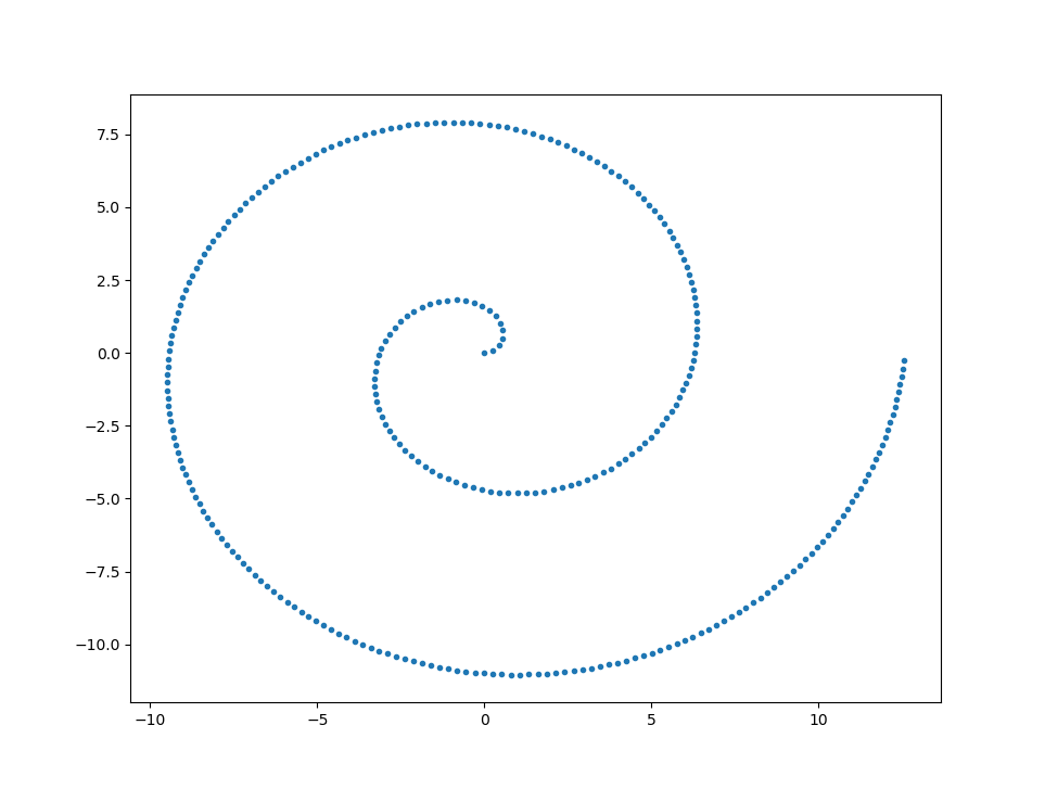
方案3

观察到这样的事实，如果把 $f(t)=\sqrt{x’^2+y’^2}$（还需要归一化） 看成一个概率密度函数，那么就可以用蒙特卡洛方法来做了。

算法步骤：

1. 计算解析形式$f(t)=\sqrt{x’^2+y’^2} dt$
2. 计算$m=\max f(t)$ （或者m比最大值大一些也ok）
3. 在t可能的区域内随机选取一点$t$，计算$f(t)/m$
4. 生成一个随机数$r\in [0,1]$，如果$f(x)/m>r$，则保留x，否则丢弃x并回到2

代码

import scipy.optimize as opt
import numpy as np


def func(t):
    # 被积部分
    return np.sqrt(1 + np.square(t))


left, right = 0, 4 * np.pi
m = -opt.minimize(fun=lambda t: -func(t), x0=np.array([0.1]),
                  method=None, jac=None,
                  bounds=((left, right),)).fun[0]

t_list = []
for i in range(1000):
    t = np.random.rand() * (right - left) + left
    if func(t) / m > np.random.rand():
        t_list.append(t)

x = t_list * np.cos(t_list)
y = t_list * np.sin(t_list)
plt.plot(x, y, '.')
plt.show()

优缺点：

• 不用解积分，也不用解方程。大大提高效率
• 但是会有大量空运算（丢弃），所以当f不均匀，或者返回太大时，效率变低。不过貌似效率再低也比方案2强。

这是目前能想到的最有效的方案了。

曲面上的均匀随机

推广

回到曲线上均匀分布的推导过程，我们找到方程 $\dfrac{\int_{a}^{x} ds}{\int_{a}^{b} ds}=r$，其中$r\in[0,1]$ 的解，作为随机生成算法。
由于积分和方程难以解出，求助了数值方法去计算。

对于曲面上的情况，类似的，
$\iint_D 1d\sigma=\iint_{\Omega_{xy}}\sqrt{1+(\dfrac{\partial z}{\partial x})^2+(\dfrac{\partial z}{\partial y})^2}dxdy=r$

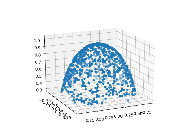
案例：球面

$z=\sqrt{1-x^2-y^2}$

$f(x,y)=\sqrt{1+(\dfrac{\partial z}{\partial x})^2+(\dfrac{\partial z}{\partial y})^2}=\sqrt{1/(1-x^2-y^2)}$

为了符号统一，我们把$f(x,y)$定义在$R^2$上，并且对于原本没有定义的点，定义$f(x,y)=0$
不影响积分$\int_{-\infty}^{+\infty}\int_{-\infty}^{+\infty} f(x,y)dxdy$

又记 $g(x)=\int_{-\infty}^{+\infty} f(x,y)dy$
得到$\int_{-\infty}^{x}g(x)/\int_{-\infty}^{+\infty}g(x)=r$，并求解$x=x’$
$\int_{-\infty}^{y} f(x’,y)dy/\int_{-\infty}^{+\infty} f(x’,y)dy=r’$，求解$y=y’$

之后得到$(x’,y’)$就是我们要的结果

from scipy import optimize as opt
from scipy import integrate
import numpy as np
import matplotlib.pyplot as plt
from mpl_toolkits.mplot3d import Axes3D

fig = plt.figure()
ax = fig.gca(projection='3d')


def bound(x, y):
    return x ** 2 + y ** 2 <= 0.9


def func(x, y):
    if bound(x, y):
        return 1 / np.sqrt(1 - x ** 2 - y ** 2)
    else:
        return 0


x_min, x_max, y_min, y_max = -0.9, 0.9, -0.9, 0.9


def func_g(x):
    g = integrate.quad(lambda y: func(x, y), -np.sqrt(1 - x ** 2), np.sqrt(1 - x ** 2))
    return g[0]


# g(x)的最大值
m1 = -opt.minimize(fun=lambda x: -func_g(x), x0=np.array([0.1]),
                   bounds=((x_min, x_max),)).fun
# f(x,y)的最大值
# m2 = -opt.minimize(fun=lambda xy: -func(xy[0], xy[1]), x0=np.array([0.1, 0.1]),
#                    bounds=((x_min, x_max), (y_min, y_max))).fun

m2 = np.sqrt(10)

result = []
for i in range(1000):
    x = np.random.rand() * (x_max - x_min) + x_min
    if func_g(x) / m1 > np.random.rand():
        not_find = True
        while not_find:
            y = np.random.rand() * (y_max - y_min) + y_min
            if func(x, y) / m2 > np.random.rand():
                result.append([x, y])
                not_find = False

# 整理并绘图
result = np.array(result)

X = result[:, 0]
Y = result[:, 1]
Z = np.sqrt(1 - X ** 2 - Y ** 2)
surf = ax.scatter(X, Y, Z)
plt.show()

# %%
np.array([func_g(i) for i in np.arange(-1, 1, 0.1)])

缺点与改进

上面的程序warning很多，这是因为边缘太陡峭了，导致偏导数很大。另外如果边缘陡峭，算法效率也很低，因为大多数区域内的取样大概率被剔除，然后重新取样。

为了解决这个问题，考虑把曲面方程变成参数形式（曲线线的情况就是这么干的）。

假设我们的曲面方程式这个形式 $\vec r=\vec r(u,v)$
曲面积分为 $\iint_{D}=\mid\vec r_u\times\vec r_v\mid dudv$

推导过程就不写了，直接上算法流程

1. 对于通常的曲面可以（并不）轻松地找到上述参数表示形式，使得：
   • $\vec r_u\times\vec r_v \neq 0$
   • $u,v$的边界都是常数（而不是互相有关）
2. 计算 $I(u,v)=\mid\vec r_u\times\vec r_v\mid$
3. 计算 $m=\max I+\delta$（其中$\delta\geq0$可以自行制定，如果对m的计算没有信心，可以指定为一个正数，这个数如果太大，算法效率会有所降低。）
4. 对$u,v$在其边界内均匀采样，并且以$I(u,v)/m$的概率丢弃这次采样结果

以球面为例$\vec r=(\sin u\cos v,\sin u\sin v,\cos u)$

import numpy as np
import scipy.optimize as opt
from scipy.misc import derivative


# 参数方程$r=r(u,v)$
def func(u, v):
    x = np.sin(u) * np.cos(v)
    y = np.sin(u) * np.sin(v)
    z = np.cos(u)
    return x, y, z


# r对u的偏导数，可以手算，这里用数值方法
def func_r_u(u, v):
    return derivative(lambda u: func(u, v)[0], u), \
           derivative(lambda u: func(u, v)[1], u), \
           derivative(lambda u: func(u, v)[2], u)


# r对v的偏导数
def func_r_v(u, v):
    return derivative(lambda v: func(u, v)[0], v), \
           derivative(lambda v: func(u, v)[1], v), \
           derivative(lambda v: func(u, v)[2], v)


def func_I(u, v):
    r_u = func_r_u(u, v)
    r_v = func_r_v(u, v)
    E = np.linalg.norm(r_u, ord=2)
    G = np.linalg.norm(r_v, ord=2)
    F = np.dot(r_u, r_v)
    return np.sqrt(E * G - F ** 2)


left, right = 0, 2 * np.pi
m = -opt.minimize(fun=lambda t: -func_I(t[0], t[1]), x0=np.array([0.1, 0.1]),
                  bounds=((left, right), (left, right))).fun

m = m + 0.1
# %%
points = np.random.rand(3000, 2) * np.pi * 2
result = []
for point in points:
    if func_I(point[0], point[1]) / m > np.random.rand():
        result.append(point)

# %%画图

import matplotlib.pyplot as plt
from mpl_toolkits.mplot3d import Axes3D

fig = plt.figure()
ax = fig.gca(projection='3d')

X, Y, Z = [], [], []
for point in result:
    u, v = point
    x, y, z = func(u, v)
    X.append(x)
    Y.append(y)
    Z.append(z)

X = np.array(X)
Y = np.array(Y)
Z = np.array(Z)

surf = ax.scatter(X, Y, Z, '.')
plt.show()

优点：

1. 参数的边界是方形的，用$z(x,y)$表示的球面，其x-y边界不是方形的。
2. 参数可以尽量避免偏导数过大，甚至无穷大的情况