【OpenCV2】滤波器、边缘、轮廓
🗓 2020年03月07日 📁 文章归类: 0x25_CV
版权声明:本文作者是郭飞。转载随意,标明原文链接即可。
原文链接:https://www.guofei.site/2020/03/07/cv2.html
空间滤波
不同的书会有不同的叫法,空间滤波器、卷积滤波器、卷积模版、卷积核。这里不严格区分。
卷积操作 $g(x,y)=\sum\limits_{s=-a}^a\sum\limits_{s=-b}^b w(s,t)f(x+s,y+t)$
- $w(s,t)$是卷积核的情况,并且已经旋转了180度了
- 卷积核的大小是$(2a+1,2b+1)$
均值滤波器
又叫平滑线性滤波器
例如,\(\left [ \begin{array}{ccc} 1/9&1/9&1/9\\ 1/9&1/9&1/9\\ 1/9&1/9&1/9\\ \end{array}\right]\)
这个卷积核的效果是让图像更平滑
- 优点:可以用来去噪,因为典型的噪声是灰度级急剧变化造成的。
- 缺点:图像边缘也有图像灰度尖锐变化的特征,因此导致边缘模糊。
作为算法优化,通常可以先计算加和值,然后再乘以系数调整。
高斯滤波器
$h(x,y)=\exp{(-\dfrac{x^2+y^2}{2\sigma^2})}$
一个例子,\(\dfrac{1}{16} \times\left [ \begin{array}{ccc} 1&2&1\\ 2&4&2\\ 1&2&1\\ \end{array}\right]\)
统计排序滤波器
统计排序滤波器是一种非线性滤波器。其中一个普遍的例子是中值滤波器。
中值滤波器 提供了一种优秀的去噪效果(尤其是椒盐噪声)
最大值滤波器,最小值滤波器,乃至第n大滤波器,都偶尔有用。
边缘检测-锐化滤波器
锐化滤波器的效果是突出灰度的过渡部分,用途十分广泛。
先定义 整数函数的微分,可以有 很多种 定义,但我们希望一个定义满足以下几点:
- 恒定灰度区域的微分值为0
- 灰度台阶或斜坡处微分非零
- 沿着斜坡的微分值非零
类似希望二阶微分满足:
- 恒定区域微分值为0
- 灰度台阶或斜坡起点微分非零
- 沿着斜坡的微分值非零(?怀疑书上翻译错误)
我们定义一种微分和二阶微分:$\dfrac{\partial f}{\partial x}=f(x+1)-f(x), \dfrac{\partial^2 f}{\partial x^2}=f(x+1)+f(x-1)-2f(x)$
可以想到:物体的边缘往往类似斜面,所以一阶微分产生一个粗边缘,二阶微分产生一个双边缘,所以
- 二阶微分增强细节的能力比一阶微分更强
- 并且二阶微分执行上更容易
Sobel算子和Scharr算子
cv2.Sobel(src, ddepth, dx, dy[,ksize[, scale[, delta[, borderType]]]])
# ddepth: 0 负梯度截断为0,cv2.CV_64F 保留负梯度,同时
# dx 代表 x 方向上的求导阶数。
# dy 代表 y 方向上的求导阶数。
# 如果 dx,dy 都是1,代表斜向的导数
# ksize 代表 Sobel 核的大小。该值为-1 时,则会使用 Scharr 算子进行运算。

# 或者
kernel=np.array([[-1, 0, 1], [-2, 0, 2], [-1, 0, 1]]) # 检测水平线
kernel=np.array([[-1, - 2, - 1], [0, 0, 0], [1, 2, 1]]) # 检测垂直线
cv2.filter2D(picture, -1, kernel)
Scharr算子是对Sobel算子的改进
dst=Scharr(src, cv2.CV_64F, dx, dy)
dst= cv2.convertScaleAbs(dst)

# 或者
kernel_y = np.array([[-3, 0, 3], [-10, 0, 10], [-3, 0, 3]]) # 检测水平线
kernel_x=np.array([[-3, - 10, - 3], [0, 0, 0], [3, 10, 3]]) # 检测垂直线
cv2.filter2D(picture, -1, kernel)
拉普拉斯算子
拉普拉斯算子 是一种常用的 二阶微分滤波器 ,定义为 \(\nabla^2f=\dfrac{\partial^2 f}{\partial x^2}+\dfrac{\partial^2 f}{\partial y^2}\)
因为 任意阶微分都是线性操作,所以 拉普拉斯变换是线性算子
离散化描述:
- $\dfrac{\partial^2 f}{\partial x^2}=f(x+1,y)+f(x-1,y)-2f(x,y)$
- $\dfrac{\partial^2 f}{\partial y^2}=f(x,y+1)+f(x,y-1)-2f(x,y)$
- 所以 $\nabla^2f=f(x+1,y)+f(x-1,y)+f(x,y+1)+f(x,y-1)-4f(x,y)$
我们得到这样的滤波器:
\(\left [ \begin{array}{ccc}
0&1&0\\
1&-4&1\\
0&1&0\\
\end{array}\right]
\left [ \begin{array}{ccc}
1&1&1\\
1&-8&1\\
1&1&1\\
\end{array}\right]
\left [ \begin{array}{ccc}
0&-1&0\\
-1&4&-1\\
0&-1&0\\
\end{array}\right]
\left [ \begin{array}{ccc}
-1&-1&-1\\
-1&8&-1\\
-1&-1&-1\\
\end{array}\right]\)
经常会把二阶滤波后的图像,加到原图像上,以增强图像。这时候需要注意正负号,后两个卷积核处理后直接相加就行了。
实际操作中,还会把二阶滤波后的图像,做一个“把负灰度变成0”的操作。(感觉很像ReLU啊)
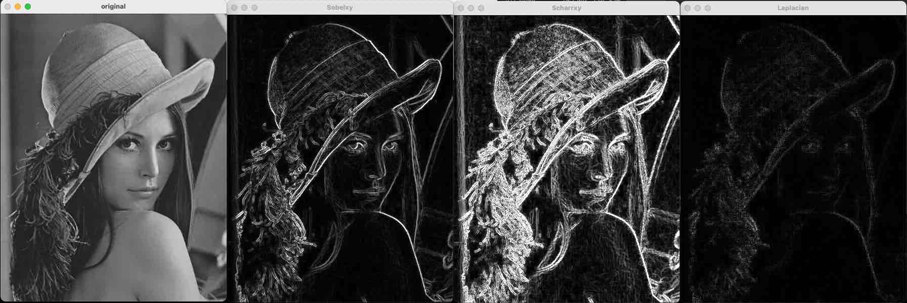
下面的代码是 Sobel+Scharr+Laplacian:
o = cv2.imread("a.jpeg", cv2.IMREAD_GRAYSCALE)

# Sobel:两个方向叠加,可以把所有方向的边界都显示出来
Sobelx = cv2.Sobel(o, cv2.CV_64F, dx=1, dy=0, ksize=3)
Sobely = cv2.Sobel(o, cv2.CV_64F, dx=0, dy=1, ksize=3)
Sobelx = cv2.convertScaleAbs(Sobelx)
Sobely = cv2.convertScaleAbs(Sobely)
Sobelxy = cv2.addWeighted(Sobelx, 0.5, Sobely, 0.5, 0)

# Scharr
Scharrx = cv2.Scharr(o, cv2.CV_64F, dx=1, dy=0)
Scharry = cv2.Scharr(o, cv2.CV_64F, dx=0, dy=1)
Scharrx = cv2.convertScaleAbs(Scharrx)
Scharry = cv2.convertScaleAbs(Scharry)
Scharrxy = cv2.addWeighted(Scharrx, 0.5, Scharry, 0.5, 0)

# Laplacian
Laplacian = cv2.Laplacian(o, cv2.CV_64F)
Laplacian = cv2.convertScaleAbs(Laplacian)

cv2.imshow("original", o)
cv2.imshow("Sobelxy", Sobelxy)
cv2.imshow("Scharrxy", Scharrxy)
cv2.imshow("Laplacian", Laplacian)
cv2.waitKey()
cv2.destroyAllWindows()
其它滤波器
kernel = cv2.getStructuringElement(cv2.MORPH_RECT, (5, 5))  # 矩形结构
kernel = cv2.getStructuringElement(cv2.MORPH_ELLIPSE, (5, 5))  # 椭圆结构
kernel = cv2.getStructuringElement(cv2.MORPH_CROSS, (5, 5))  # 十字形结构
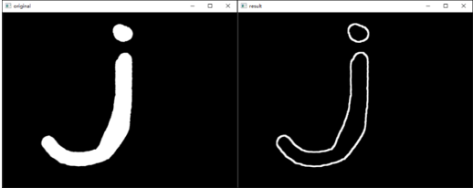
Canny 边缘检测
Canny 边缘检测分为如下几个步骤:
- 步骤 1:去噪。噪声会影响边缘检测的准确性,因此首先要将噪声过滤掉。例如用高斯滤波器
- 步骤 2:计算梯度的幅度与方向:$G=\sqrt{G_x^2+G_y^2}; \theta=arctan(G_y/G_x)$,通常取8个方向。
- 步骤 3:非极大值抑制,即适当地让边缘“变瘦”。遍历像素点,去除非边缘的点。
- 如果该点是同梯度方向(正或负)上的局部最大值,则保留该点。
- 如果不是,则抑制该点(归零)。
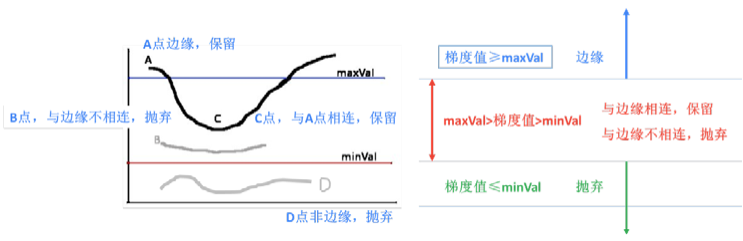
- 步骤 4:确定边缘。使用双阈值算法确定最终的边缘信息。设置两个阈值,其中一个为高阈值 maxVal,另一个为低阈值 minVal。
- 如果边缘像素的梯度值大于或等于 maxVal,则将当前边缘像素标记为强边缘。
- 如果当前边缘像素的梯度值小于或等于 minVal,则抑制当前边缘像素。
- 如果当前边缘像素的梯度值介于 maxVal 与 minVal 之间,则将当前边缘像素标记为虚边缘
- 与强边缘连接,则将该边缘处理为边缘。与强边缘无连接,则该边缘为弱边缘,将其抑制。
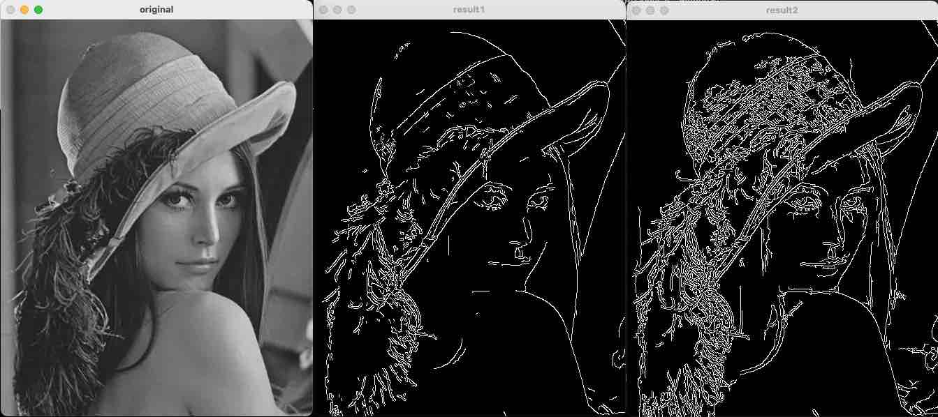
用法
# edges = cv.Canny( image, threshold1, threshold2[, apertureSize[, L2gradient]])

o = cv2.imread("a.jpeg", cv2.IMREAD_GRAYSCALE)
r1 = cv2.Canny(o, 128, 200)
r2 = cv2.Canny(o, 32, 128)
cv2.imshow("original", o)
cv2.imshow("result1", r1)
cv2.imshow("result2", r2)
cv2.waitKey()
cv2.destroyAllWindows()
轮廓检测
image, contours, hierarchy = cv2.findContours(image, mode, method)
注意:findContours 只接受二值图,所以效果的好坏取决于你的二值图是怎么做出来的
入参:
- mode
- cv2.RETR_EXTERNAL 表示只检测外轮廓
- cv2.RETR_LIST 检测的轮廓不建立等级关系
- cv2.RETR_CCOMP 建立两个等级的轮廓,上面的一层为外边界,里面的一层为内孔的边界信息。如果内孔内还有一个连通物体,这个物体的边界也在顶层。
- cv2.RETR_TREE 建立一个等级树结构的轮廓。
- mothod
- mothod=cv2.CHAIN_APPROX_NON,输出的是轮廓所有的坐标点
- mothod=cv2.CHAIN_APPROX_SIMPLE,只会输出4个顶点
- cv2.CHAIN_APPROX_TC89_L1,CV_CHAIN_APPROX_TC89_KCOS使用teh-Chinl chain 近似算法
img = cv2.imread('img_b.jpg')
img_gray = cv2.cvtColor(img, cv2.COLOR_BGR2GRAY)  # 变成灰度
retval, dst = cv2.threshold(img_gray, thresh=127, maxval=255, type=0)  # 二值化
contours, hierarchy = cv2.findContours(image=dst, mode=cv2.RETR_TREE, method=cv2.CHAIN_APPROX_SIMPLE)

# contours:列表,每个元素是个array,每个轮廓的坐标点的(x, y)的Numpy数组。
# hierarchy 是一个三维数组,它储存了所有等高线(轮廓)的层级结构
绘制轮廓
img_with_contours = cv2.drawContours(image=img, contours=contours, contourIdx=-1, color=(0, 255, 0), thickness=5)

cv2.imshow("img_with_contours", img_with_contours)
cv2.waitKey()
cv2.destroyAllWindows()
下面几个参数都很重要:
- contourIdx 列表索引,用来选择要绘制的轮廓,为-1时表示绘制所有轮廓;
- color 是轮廓颜色
- thickness 是轮廓线的宽度,为-1时表示填充内部。-1生成的矩阵,还可以进一步用来做掩码
- 入参 img 会被修改
距特征
距特征是轮廓的一系列特征
空间距
- m00(其实是面积)
- m10,m01
- m20,m11,m02
- m30,m21,m12,m03
中心距
- mu20,mu11,mu02
- mu30,mu21,mu12,mu03
归一化中心距
- nu20,nu11,nu02
- nu30,nu21,nu12,nu03
演示:
img = cv2.imread('a.png')
img_gray = cv2.cvtColor(img, cv2.COLOR_BGR2GRAY)  # 变成灰度
retval, dst = cv2.threshold(img_gray, thresh=127, maxval=255, type=0)  # 二值化
contours, hierarchy = cv2.findContours(image=dst, mode=cv2.RETR_TREE, method=cv2.CHAIN_APPROX_SIMPLE)

n = len(contours)

contoursImg = []
for i in range(n):
    contoursImg_ = cv2.drawContours(np.zeros(img.shape, np.uint8), contours, i, 255, 3)
    contoursImg.append(contoursImg_)
    cv2.imshow("contours[" + str(i) + "]", contoursImg[i])

print("观察各个轮廓的矩(moments):")
for i in range(n):
    print("轮廓" + str(i) + "的矩:\n", cv2.moments(contours[i]))

print("观察各个轮廓的面积:")
for i in range(n):
    print("轮廓" + str(i) + "的面积:%d" % cv2.moments(contours[i])['m00'])

cv2.waitKey()
cv2.destroyAllWindows()
面积和周长
面积
for i in range(n):
    retval = cv2.contourArea(contour=contours[i], oriented=True)
    print(retval)
oriented=True 时,返回值可以为负(表示轮廓逆时针),正(表示轮廓顺时针)
周长
for i in range(n):
    retval = cv2.arcLength(curve=contours[i], closed=True)
    print(retval)
closed=True 表示这个曲线是封闭的。如果不封闭,不会计算末尾到开头的那段距离。
hu距
Hu 矩在图像旋转、缩放、平移等操作后,仍能保持矩 的不变性,所以经常会使用 Hu 距来识别图像的特征。
Hu 距是用 moments 的结果按照某个公式计算出来的
cv2.HuMoments(cv2.moments(img_gray))
ret0 = cv2.matchShapes(contours[0], contours[1], 1, 0.0)
ret1 = cv2.matchShapes(contours[0], contours[2], 1, 0.0)
ret2 = cv2.matchShapes(contours[1], contours[2], 1, 0.0)
print("0与1的相似度:", ret0)
print("0与2的相似度:", ret1)
print("1与2的相似度:", ret2)
这个相似度无视大小、位置、旋转
- 值越小,越相似
- 实测大小更接近的话,相似度也会稍微变小?
使用素材:
轮廓拟合
有 contour 的情况下,还可以找到外接矩形等
准备:提取轮廓
o = cv2.imread('tst_contour.png')

# 提取轮廓
gray = cv2.cvtColor(o, cv2.COLOR_BGR2GRAY)
ret, binary = cv2.threshold(gray, 127, 255, cv2.THRESH_BINARY)
contours, hierarchy = cv2.findContours(binary, cv2.RETR_LIST, cv2.CHAIN_APPROX_SIMPLE)
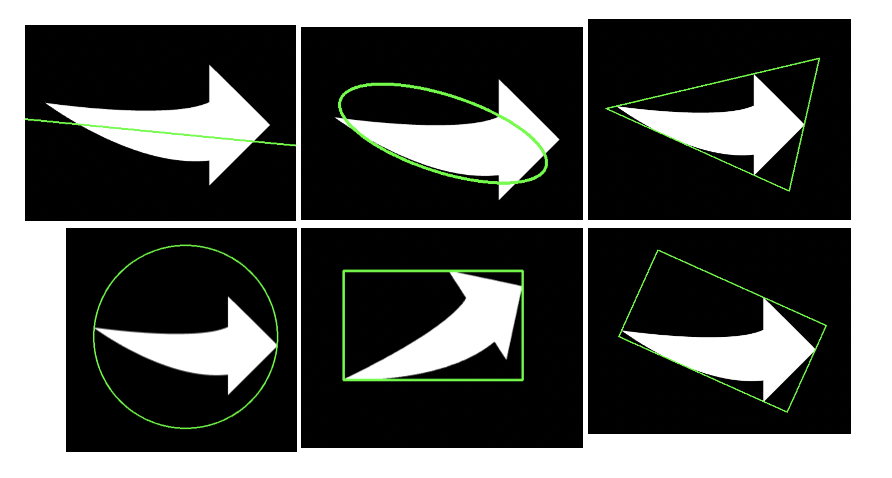
外框矩形(指的是不旋转的外接矩形)
x, y, w, h = cv2.boundingRect(contours[2])
brcnt = np.array([[[x, y]], [[x + w, y]], [[x + w, y + h]], [[x, y + h]]])
bounding_rect = copy.deepcopy(o)
cv2.drawContours(bounding_rect, [brcnt], -1, (0, 255, 0), 2)
cv2.imshow("bounding rect", bounding_rect)
外接矩形(旋转的外接矩形)
rect = cv2.minAreaRect(contours[0])
# rect 的结构是(最小外接矩形的中心(x,y),(宽度,高度),旋转角度)
points = cv2.boxPoints(rect)
# 获取边界点
min_rect = copy.deepcopy(o)
cv2.drawContours(min_rect, [np.int0(points)], -1, (0, 255, 0), 2)
cv2.imshow("min rect", min_rect)
外接圆
(x, y), radius = cv2.minEnclosingCircle(contours[0])
min_circle = copy.deepcopy(o)
cv2.circle(min_circle, (int(x), int(y)), int(radius), (0, 255, 0), 2)
cv2.imshow("min circle", min_circle)
拟合椭圆
ellipse = cv2.fitEllipse(contours[0])  # 椭圆的中心、轴、旋转角度
min_ell = copy.deepcopy(o)

cv2.ellipse(min_ell, ellipse, (0, 255, 0), 3)
cv2.imshow("min_ell", min_ell)
拟合直线
fit_line = copy.deepcopy(o)
rows, cols = o.shape[:2]
[vx, vy, x, y] = cv2.fitLine(contours[0], cv2.DIST_L2, 0, 0.01, 0.01)
lefty = int((-x * vy / vx) + y)
righty = int(((cols - x) * vy / vx) + y)
cv2.line(fit_line, (cols - 1, righty), (0, lefty), (255, 255, 255), 2)

cv2.imshow("fit line", fit_line)
外接三角形
area, trgl = cv2.minEnclosingTriangle(contours[0])  # 返回值:面积,三个顶点坐标

tri = copy.deepcopy(o)
trgl = trgl.astype(np.int)
for i in range(0, 3):
    cv2.line(tri, tuple(trgl[i][0]),
             tuple(trgl[(i + 1) % 3][0]), (0, 255, 0), 2)
cv2.imshow("tri", tri)
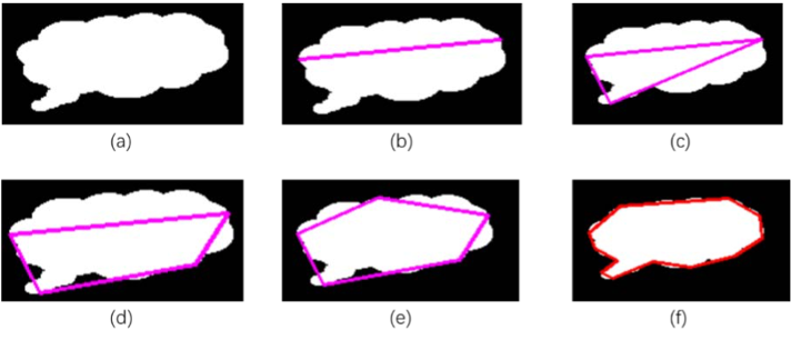
多边形逼近
- cv2.approxPolyDP()采用的是 Douglas-Peucker 算法(DP 算法)。
- 该算法首先从轮廓中找到距离最远的两个点,并将两点相连(见图 12-23 的(b)图)。接下来,在 轮廓上找到一个离当前直线最远的点,并将该点与原有直线连成一个封闭的多边形,此时得到 一个三角形。
将上述过程不断地迭代,将新找到的距离当前多边形最远的点加入到结果中。
o = cv2.imread('tst_contour.png')
cv2.imshow("original", o)
gray = cv2.cvtColor(o, cv2.COLOR_BGR2GRAY)
ret, binary = cv2.threshold(gray, 127, 255, cv2.THRESH_BINARY)

contours, hierarchy = cv2.findContours(binary,
                                       cv2.RETR_LIST,
                                       cv2.CHAIN_APPROX_SIMPLE)
# ----------------epsilon=0.1*周长-------------------------------
adp = o.copy()
epsilon = 0.1 * cv2.arcLength(contours[0], True)

approx = cv2.approxPolyDP(contours[0], epsilon, True)
adp = cv2.drawContours(adp, [approx], 0, (0, 0, 255), 2)
cv2.imshow("result0.1", adp)
# ----------------epsilon=0.09*周长-------------------------------
adp = o.copy()
epsilon = 0.09 * cv2.arcLength(contours[0], True)
approx = cv2.approxPolyDP(contours[0], epsilon, True)
adp = cv2.drawContours(adp, [approx], 0, (0, 0, 255), 2)
cv2.imshow("result0.09", adp)
# ----------------epsilon=0.055*周长-------------------------------
adp = o.copy()
epsilon = 0.055 * cv2.arcLength(contours[0], True)
approx = cv2.approxPolyDP(contours[0], epsilon, True)
adp = cv2.drawContours(adp, [approx], 0, (0, 0, 255), 2)
cv2.imshow("result0.055", adp)
# ----------------epsilon=0.05*周长-------------------------------
adp = o.copy()
epsilon = 0.05 * cv2.arcLength(contours[0], True)
approx = cv2.approxPolyDP(contours[0], epsilon, True)
adp = cv2.drawContours(adp, [approx], 0, (0, 0, 255), 2)
cv2.imshow("result0.05", adp)
# ----------------epsilon=0.02*周长-------------------------------
adp = o.copy()
epsilon = 0.02 * cv2.arcLength(contours[0], True)
approx = cv2.approxPolyDP(contours[0], epsilon, True)
adp = cv2.drawContours(adp, [approx], 0, (0, 0, 255), 2)
cv2.imshow("result0.02", adp)

cv2.waitKey()
cv2.destroyAllWindows()
凸包
hull = cv2.convexHull( points[, clockwise[, returnPoints]] )

# 凸缺陷:距离凸包最远的凹陷
convexityDefects = cv2.convexityDefects( contour, convexhull )
几何学测试
- 轮廓是否凸:
cv2.isContourConvex() - 点到轮廓的距离:
cv2.pointPolygonTest()有正负,代表点在内部还是外部
轮廓相似性
sd = cv2.createShapeContextDistanceExtractor()
d1 = sd.computeDistance(contour1,contour2)
Hausdorff距离
hd = cv2.createHausdorffDistanceExtractor()
hd.computeDistance(contour1,contour2)
cv2实现滤波
kernel=np.array([[-1, -1, -1], [-1, 8, -1], [-1, -1, -1]]) # 边缘检测,元素之和倾向于0,所以图像会很暗

kernel=np.array([[-1, -1, -1], [-1, 9, -1], [-1, -1, -1]]) # 锐化

kernel = np.array([[1, 1, 1], [1, -7, 1], [1, 1, 1]])  # 边缘检测

# Sobel算子
kernel=np.array([[-1, 0, 1], [-2, 0, 2], [-1, 0, 1]]) # 检测水平线
kernel=np.array([[-1, - 2, - 1], [0, 0, 0], [1, 2, 1]]) # 检测垂直线


kernel = np.array([[-2, -2, -2, -2, 0],
                   [-2, -2, -2, 0, 2],
                   [-2, -2, 0, 2, 2],
                   [-2, 0, 2, 2, 2],
                   [0, 2, 2, 2, 2]])  # 浮雕,然后用 cvtColor 转成灰度图像


cv2.filter2D(picture, -1, kernel)
参考:https://blog.csdn.net/u013421629/article/details/78899828
另有一篇也是滤波器的:https://www.cnblogs.com/zyly/p/8893579.html
滤波
- 均值滤波
cv2.blur( src, ksize, anchor, borderType)ksize滤波核大小anchor默认 (-1, -1) 表示均值点位于滤波核的中心borderType边界样式
- 方框滤波
cv2.boxFilter - 中值滤波
dst = cv2.medianBlur( src, ksize)
双边滤波
前面的滤波器会让图像边界变得模糊,双边滤波在计算时,会考虑:
- 距离信息:距离越远、权重越小
- 色彩信息:颜色差别越大,权重越小
所以它能去除噪声的同时,较好的保护边缘信息
dst = cv2.bilateralFilter( src, d, sigmaColor, sigmaSpace, borderType)
用TF实现滤波
用TensorFlow来做,因为滤波器是每层独立滤波的,所以用for loop处理一下
import cv2
import numpy as np
import tensorflow as tf

capture = cv2.VideoCapture(0)
sess = tf.Session()

kernel=np.array([[-1, - 2, - 1], [0, 0, 0], [1, 2, 1]]) # 检测水平线
f_1, f_2 = kernel.shape
kernel_tf = np.zeros((f_1, f_2, 3, 3))
for i in range(3):
    kernel_tf[:, :, i, i] = kernel

width, height = capture.get(3), capture.get(4)
x = tf.placeholder(dtype=tf.float32, shape=(None, height, width, 3))
sess.run(tf.global_variables_initializer())
# %%
while (True):
    ret, picture = capture.read()
    # ret 是布尔值,表示当前帧是否正确;picture是np.array

    a = tf.nn.conv2d(x, kernel_tf, strides=[1, 1, 1, 1], padding='SAME')
    a_value = sess.run(a, feed_dict={x: [picture]})
    cv_conv = cv2.filter2D(picture, -1, kernel)

    cv2.imshow('origin', picture)
    cv2.imshow('tf_conv', a_value[0] / 256)
    cv2.imshow('cv_conv', cv_conv)
    if cv2.waitKey(1) == ord('q'):
        break

cv2.destroyAllWindows()
capture.release()
形态学
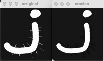
腐蚀
- 相当于一种“最小值滤波”
- 边界被缩小“像腐蚀一样”
- 毛刺消失
img = cv2.imread("c.png", 0)
kernel = np.ones((5, 5), np.uint8)
erosion = cv2.erode(img, kernel)
膨胀
与腐蚀相比是逆操作
kernel = np.ones((5, 5), np.uint8)
erosion = cv2.dilate(img, kernel, iterations=3)
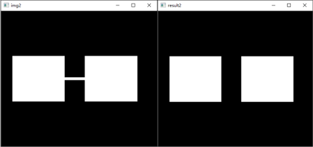
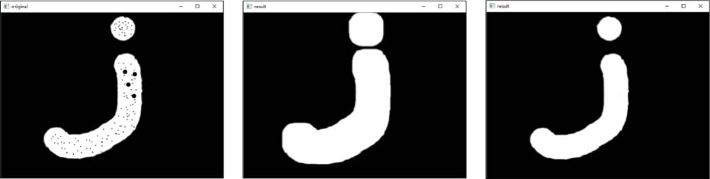
开运算和闭运算
开运算:先腐蚀后膨胀,用于去噪、去毛刺、去除物体之间的连接
k=np.ones((10,10),np.uint8)
r1=cv2.morphologyEx(img1,cv2.MORPH_OPEN,k)
闭运算:先膨胀后腐蚀,用于去除物体内的孔洞、合并临接物体
closing = cv2.morphologyEx(img, cv2.MORPH_CLOSE, kernel)
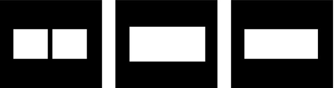
梯度运算、礼帽运算、黑帽运算
膨胀图像减腐蚀图像,可以获得边缘
r=cv2.morphologyEx(o,cv2.MORPH_GRADIENT,k)
- 原始图像减去开运算,可以获得噪声
cv2.morphologyEx(img, cv2.MORPH_TOPHAT, kernel)
- 黑帽运算是用闭运算图像减去原始图像的操作,可以获得图像内部的小孔,以及
cv2.morphologyEx(o2,cv2.MORPH_BLACKHAT,k)
图像金字塔
- 下采样
cv2.pyrDown会减少分辨率:先高斯滤波,然后间隔采样,分辨率减半 - 上采样,
cv2.pyrUp会增加分辨率:对行和列插入零,然后高斯滤波,乘以4
下采样和上采样不是可逆的运算,他们之间的差别叫做 拉普拉斯金字塔
您的支持将鼓励我继续创作!